VB code to list names of all worksheets present in a workbook

Sub ListSheetNames()
Dim Wsheet As Worksheet
Dim Rownumber As Integer
Rownumber = 1
'Intialize the row in which the name listing would start'
Sheets("INDEX").Range("A:A").Clear
'Clear any data previously present in column A'
For Each Wsheet In Worksheets
Sheets("INDEX").Cells(Rownumber, 1) = Wsheet.Name 

'List all the names of sheets present in the workbook in Column A (1)' 

Rownumber = Rownumber + 1
'Increment the row value for continuous listing'
Next Wsheet
End Sub

Copy this code into a new module in the Visual Basic Editor(Alt+F11).
You could further create a drop down list of sheet names by using this data. For how to create a drop down list please see  
How to create a drop down list using data validation?

 

How to use sumif formula?

Sumif is a summing operation that adds only those values which meet a required condition. The condition to be met may be in a same column or row or in a different column or row. The syntax for Sumif formula is as follows:

1. Criteria indicates the condition put forth by the user which needs to be looked for in a particular column or row.

2.  Range indicates the range of rows or column in which the criteria needs to be looked up and satisfied.

3.  Sum_range is the range of values that needs to be summed if the criteria is found in the Range. The Sum-range can be the Range itself or it can be other cells corresponding to the Range columns or rows.

Lets now go through an example.

I have a table which is used to enter time required for 4 different processes. the column E is used to calculate the total of the entries in the columns B, C and D respectively. Now my requirement is to get the total of individual processes in the grid arrangement on the top two rows 1 and 2. And there is no better option than to use Sumif option in this case

Now following the syntax of the Sumif formula, In the cell C1 type the following: =SUMIF(A5:A18,"DETAILING",E5:E18)

 Similarly modify the above shown formula in the other 3 cells by changing the process names. 

=SUMIF(A5:A18,"FINAL CHECK",E5:E18)

=SUMIF(A5:A18,"SELF CHECK",E5:E18)

=SUMIF(A5:A18,"ENGINEERING",E5:E18)

  Enter some values under respective cells and check.

Try it!

How to automatically add a new sheet and Hyper link it to an Index sheet?

Those who know basics in excel do know how to hyper link different sheets within a workbook. But I am still going to brush up! 

What is a hyper link?

A hyper link is a reference to a document that the reader can directly follow.

Hyper links are generally useful when there are many sheets in a single workbook. This allows a 

degree of flexibility to navigate through the sheets from a single point.

How to create a manual hyperlink?

I have a worksheet with three sheets named after the first three months of the year. Now I want to hyperlink from another sheet named Index.

Right click on any of the cells and select Hyperlink.

Select 'Place in this document' option and click on the respective sheet on the dialog box. The hyperlink is created.

Imagine creating manual hyperlinks to many such sheets. Its going to consume some time and patience of yours! So to make it a bit more exciting Visual Basic comes into picture.

To use this option I primarily need some setup!

1. A source for the name of the sheet

2. A VB code (Macro)

3. A button to activate the Macro.

In the snapshot below I have used cell B1 of the Index sheet as a place where I will enter the name of the to be generated sheet. I have used the shapes option to create a button. I will later assign a macro to this button.

Press Alt+F11. You will enter the Visual Basic Editor.

Go to Insert and select module.

Paste the following code under it.

For those of you who are new to VB check out the procedure at http://excellence2007.blogspot.com/2010/11/how-to-convert-numerical-value-to-words.html

-----------------------------------------------------------------------------------------------------------------------------------

Sub AddHyperlinkedSheet()

Sheetname1 = Worksheets("INDEX").Cells(1, "B").Value

'THE SHEET NAME TO BE GENERATED IS ENTERED IN CELL B1 OF THE INDEX SHEET'

If Worksheets("INDEX").Cells(1, "B").Value = "" Then Exit Sub

'IF THERE IS NO NAME PRESENT IN CELL B1 THEN EXIT THE CODE'

If Application.WorksheetFunction.CountIf(Worksheets("INDEX").Range("A:A"), Worksheets("INDEX").Cells(1, "B").Value) > 0 Then Exit Sub

'IF THERE IS ALREADY A SIMILAR NAME PRESENT IN COLUMN A THEN EXIT THE CODE'

Sheetname2 = Replace(Sheetname1, " ", "_")

'IF THERE ARE ANY BLANK SPACES IN THE NAME ENTERED IN CELL B1, REPLACE IT WITH UNDERSCORES'

Sheets.Add After:=Sheets("INDEX")

'IF THE NAME IS UNIQUE THEN GENERATE A SHEET AFTER THE INDEX SHEET'

ActiveSheet.Name = Sheetname2

'THE NEW SHEET WILL BE RENAMED PER THE NAME TYPED IN CELL B1'

Worksheets("INDEX").Select

Rowvalue = Worksheets("INDEX").Range("a65536").End(xlUp).Offset(1, 0).Row

'CHECK FOR THE NEXT AVAILABLE ROW IN THE INDEX SHEET AND RETURN ITS VALUE'

Worksheets("INDEX").Cells(Rowvalue, "A").Select

'SELECT THE ROW UNDER COLUMN A'

ActiveSheet.Hyperlinks.Add Anchor:=Selection, Address:="", SubAddress:=Sheetname2 & "!A1"

'ADD HYPERLINK'

Worksheets("INDEX").Cells(Rowvalue, "A").Value = Left(Worksheets("INDEX").Cells(Rowvalue, "A"), Len(Worksheets("INDEX").Cells(Rowvalue, "A")) - 3)

'TRIM CELL REFERENCE FROM THE NAME'

Sheets(Sheetname2).Select

End Sub

-----------------------------------------------------------------------------------------------------------------------------------

Close the VB editor and go back to the excel sheet. On the button, right click and assign macro and click OK.

Now enter the desired name of the sheet in cell B1 and click on the button. A new sheet will be generated and a hyper link will be created in the Index sheet.

How to retrieve data from a worksheet using Indirect referencing?

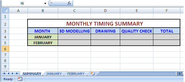
I have an example here. Lets say we have 2 sheets named January and February and a third sheet called Summary. I want the monthly total from each of the sheet to appear in the summary sheet. Now this can be done using two methods.
1. Direct referencing of worksheets
2. Indirect referencing of worksheets

In direct referencing click on a cell in the summary sheet, enter the equal (=) sign then click on the sheet and then the cell from which the data is to be retrieved. You have to do this to each of the cell in the summary table. See snapshot below.

The above method is helpful when you are summarizing data from 2 or more sheets. But what if you have plenty of such sheets. In such case indirect referencing is very helpful.
The INDIRECT function returns a reference to a range. You can use this function to create a reference that won't change if row or columns are inserted in the worksheet. Or, use it to create a reference from letters and numbers in other cells.

The INDIRECT function has two arguments:
1. ref_text: A cell reference or text string (or both), that create the range reference. The referenced range can be a cell, a range of cells, or a named range.
2. a1: Usually this value is TRUE. Refers to the type of cell referencing in excel.

The advantage with this function is that you don't need to enter the sheet name in every cell. Just enter the name of the sheet in a particular cell and then use the cell to create a reference to the actual worksheet.

The final result using either of the two methods will be as below:

INDIRECT function is a very versatile function. I will be sharing more such examples in my future blogs!

All comments and queries are welcome!!! 

Keywords: INDIRECT function, INDIRECT referencing, INDIRECT Range Reference, INDIRECT sheet reference 

How to convert numerical value to words in the Indian system?

Original Source:
http://answers.yahoo.com/question/index?qid=20071016005523AAlKbBa
To convert numerical value to words per international system please use the code from this website:
http://support.microsoft.com/default.aspx?scid=KB;EN-US;Q213360

VB Code:

Function SpellIndian(ByVal MyNumber)
Dim Rupees, Paise, Temp
Dim DecimalPlace, Count
ReDim Place(9) As String
Place(2) = " Thousand "
Place(3) = " Lakh "
Place(4) = " Crore "
Place(5) = " Arab " ' String representation of amount
MyNumber = Trim(Str(MyNumber)) ' If the number does not contain any values after the decimals the decimal point is removed'
DecimalPlace = InStr(MyNumber, ".") 'Finds the position value of . in the number entered'
If DecimalPlace > 0 Then
Paise = GetTens(Left(Mid(MyNumber, DecimalPlace + 1) & "00", 2))
MyNumber = Trim(Left(MyNumber, DecimalPlace - 1))
End If
Count = 1
Do While MyNumber <> ""
If Count = 1 Then Temp = GetHundreds(Right(MyNumber, 3))
If Count > 1 Then Temp = GetHundreds(Right(MyNumber, 2))
If Temp <> "" Then Rupees = Temp & Place(Count) & Rupees
If Count = 1 And Len(MyNumber) > 3 Then
MyNumber = Left(MyNumber, Len(MyNumber) - 3)
Else
If Count > 1 And Len(MyNumber) > 2 Then
MyNumber = Left(MyNumber, Len(MyNumber) - 2)
Else
MyNumber = ""
End If
End If
Count = Count + 1
Loop
Select Case Rupees
Case ""
Rupees = "No Rupees"
Case "One"
Rupees = "One Rupee"
Case Else
Rupees = "Rupees " & Rupees
End Select
Select Case Paise
Case ""
Paise = " Only"
Case "One"
Paise = " and One Paisa"
Case Else
Paise = " and " & Paise & " Paise"
End Select
SpellIndian = Rupees & Paise
End Function
'***************************************…
' Converts a number from 100-999 into text *
'***************************************…
Function GetHundreds(ByVal MyNumber)
Dim Result As String
If Val(MyNumber) = 0 Then Exit Function
MyNumber = Right("000" & MyNumber, 3) 'Convert the hundreds place
If Mid(MyNumber, 1, 1) <> "0" Then
Result = GetDigit(Mid(MyNumber, 1, 1)) & " Hundred "
End If
'Convert the tens and ones place
If Mid(MyNumber, 2, 1) <> "0" Then
Result = Result & GetTens(Mid(MyNumber, 2))
Else
Result = Result & GetDigit(Mid(MyNumber, 3))
End If
GetHundreds = Result
End Function
'***************************************…
' Converts a number from 10 to 99 into text. *
'***************************************…
Function GetTens(TensText)
Dim Result As String
Result = "" 'null out the temporary function value
If Val(Left(TensText, 1)) = 1 Then ' If value between 10-19
Select Case Val(TensText)
Case 10: Result = "Ten"
Case 11: Result = "Eleven"
Case 12: Result = "Twelve"
Case 13: Result = "Thirteen"
Case 14: Result = "Fourteen"
Case 15: Result = "Fifteen"
Case 16: Result = "Sixteen"
Case 17: Result = "Seventeen"
Case 18: Result = "Eighteen"
Case 19: Result = "Nineteen"
Case Else
End Select
Else ' If value between 20-99
Select Case Val(Left(TensText, 1))
Case 2: Result = "Twenty "
Case 3: Result = "Thirty "
Case 4: Result = "Forty "
Case 5: Result = "Fifty "
Case 6: Result = "Sixty "
Case 7: Result = "Seventy "
Case 8: Result = "Eighty "
Case 9: Result = "Ninety "
Case Else
End Select
Result = Result & GetDigit _
(Right(TensText, 1)) 'Retrieve ones place
End If
GetTens = Result
End Function
'***************************************…
' Converts a number from 1 to 9 into text. *
'***************************************…
Function GetDigit(Digit)
Select Case Val(Digit)
Case 1: GetDigit = "One"
Case 2: GetDigit = "Two"
Case 3: GetDigit = "Three"
Case 4: GetDigit = "Four"
Case 5: GetDigit = "Five"
Case 6: GetDigit = "Six"
Case 7: GetDigit = "Seven"
Case 8: GetDigit = "Eight"
Case 9: GetDigit = "Nine"
Case Else: GetDigit = ""
End Select
End Function

How to use this User defined function?
1. Open the excel workbook where you want this function to work.
2. Press Alt+F11. You will enter the visual basic editor

3. Click on the insert tab and select Module. Paste the above code in it.

4. Save and close the Visual Basic editor
5. Go to the worksheet and type =SpellIndian(Cellreference) in any cell where you want the result to appear.

How to lookup data while satisfying multiple conditions?

I had shown how to retrieve data from a database by looking up a single condition in my previous blog!
How to use VLOOKUP formula?

Many a times we come across situations where data retrieval depends on multiple conditions. A good example I can think of being a mechanical engineer is the selection of a screw. Screw is a threaded fastener. For one particular type of Screw the Thread/Inch and Length differs. 

Now I want to determine the inventory of a particular screw. For this I need to lookup all three values. But in Excel there is a provision to provide a single lookup value, or say a single cell reference.
So whats the solution? Simple! Combine the Screw size, Thread/Inch and the Length using a simple formula and let the result appear on a cell in the respective rows.

I have added the formula after the Length column. The result would be as shown below

I have combined the size, threads/inch and length values and separated each of them with a -

Now the next step is to create a Table to lookup the values from these database.

For that Go to the Sheet1 and rename it as LOOKUP ( you can rename anything you want). Create a table as shown, allowing the user to input data of the screw. Add a combine value cell using the same formula that I used before. Add the VLOOKUP formula under the diameter, inventory and price headers.

Thats about it! When you enter data in the input the formula gives out the respective values in the output if the data matches in the database.

For further refining your lookup table you could add drop down list of Inputs for the user to select. This will give a sophisticated look to your spreadsheet.

Leave your comments!

Keywords: Multiple Lookup, Vlookup for 2 or more conditions

How to use Format as Table?

The presentation or the look of the spreadsheet is a very important factor to be considered. Using aesthetic colors and proper borders enrich the spreadsheet. Creating tables is one of the most popular methods of presenting data. In Excel there are a wide variety of options from which you could create good tables. But if You are in a hurry the best option you could use is the "Format as Table" option.


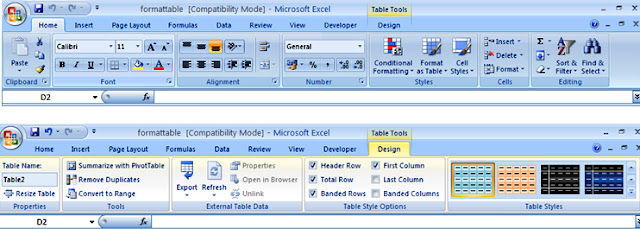
Format as table option is one of the most easiest ways of creating tables. The button can be found in the mid section of the ribbon under the Home tab.

When you click on the button a menu appears displaying a huge variety of colors that you can pick from, for creating a table.

When you select a particular color a dialog box appears. Select the range of cells on which you want the table to be formatted.

Now that you have your table created! Click anywhere on the table. A new tab called the Table tools will get highlighted on the ribbon.

You could change the style of the table by selecting from Table Styles menu.

The header row is used for classifying the columns, They come along with data filter. Un-check the Header Row if you do not need them.
You could include a row for totalling the values entered in the table. Now this Total Row option is truly versatile.You could carry out mathematical functions such as Sum, Average, Standard Deviation, Count ( Number of values entered in a column) Max (Maximum value in a column) Min (Minimum value in a column) so on.

Remove duplicates are used to remove repetitive values from a column.

Suppose you want to remove the Format Table link form the created table you could select "Convert to range". It will remove the data filter and the Format table link. This will turn out to be a simple table on range of cells.


Try other designs! Play with all the colors!