How to use VLOOKUP formula?

In Excel, the VLOOKUP formula searches for value in the left-most column of table_array and returns the value in the same row based on the index.

Didn't get it eh?

Consider a student database of a particular class in an engineering college.

The placement officer has requested the students to enter their details across rows under specified columns.

The student have entered their university seat numbers in the first column and subsequent data in other.

Say there were 100 students in the class. If each of the student has made an entry of data, then the excel sheet would turn out to be one huge pile of data.

The placement officer would have a tough time in segregating data. Now wouldn't it be easy if he could generate data in the form of a table for a particular student. These is where VLOOKUP comes to help. The syntax for VLOOKUP is:

What is a lookup_value?

It is a key for finding other data, In this example I use the University seat number as a lookup_value

What is a table_array?

It is the entire range of cells that contain the data

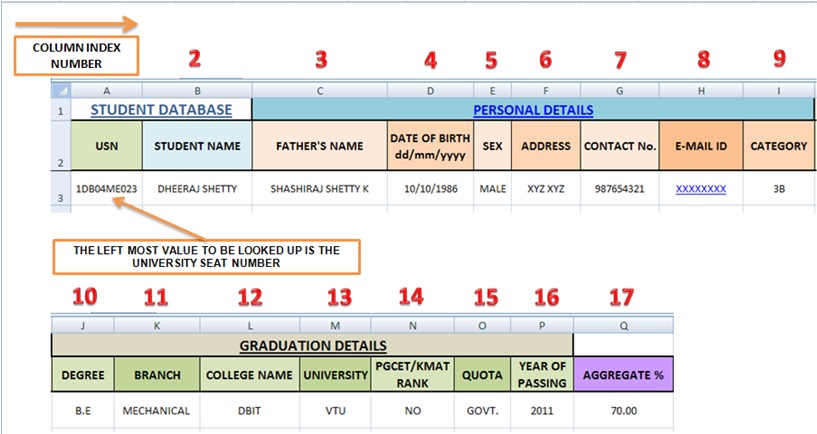
What is a column index number?

See snapshot shown below

Range_Lookup?

It should be FALSE for an exact match and TRUE for an approximate match.

Now that we have understood the syntax we will apply the VLOOKUP
I have created a Lookup worksheet containing a organized table for the data to be retrieved. In each of the specified cells I enter formulas as shown.

Interpretation of the formula beside student name.
=VLOOKUP($C$2,DATABASE!$A$3:$T2000,2,FALSE)
It says if C2 contains a university seat number, then retrieve data from the second column of table range A3:A2000 from the DATABASE worksheet by looking up the number in the left most column.


Now when I enter the university seat number in cell C2, we get!!

Try entering many such data into the database sheet and check with the Lookup sheet.

Write your comments!